40 Reports with R Markdown
R Markdown is a widely-used tool for creating automated, reproducible, and share-worthy outputs, such as reports. It can generate static or interactive outputs, in Word, pdf, html, powerpoint, and other formats.
An R Markdown script intersperces R code and text such that the script actually becomes your output document. You can create an entire formatted document, including narrative text (can be dynamic to change based on your data), tables, figures, bullets/numbers, bibliographies, etc.
Such documents can be produced to update on a routine basis (e.g. daily surveillance reports) and/or run on subsets of data (e.g. reports for each jurisdiction).
Other pages in this handbook expand on this topic:
- The page Organizing routine reports demonstrates how to routinize your report production with auto-generated time-stamped folders.
- The page Dashboards with R Markdown explains how to format a R Markdown report as a dashboard.
Of note, the R4Epis project has developed template R Markdown scripts for common outbreaks and surveys scenarios encountered at MSF project locations.
40.1 Preparation
Background to R Markdown
To explain some of the concepts and packages involved:
- Markdown is a “language” that allows you to write a document using plain text, that can be converted to html and other formats. It is not specific to R. Files written in Markdown have a ‘.md’ extension.
- R Markdown: is a variation on markdown that is specific to R - it allows you to write a document using markdown to produce text and to embed R code and display their outputs. R Markdown files have ‘.Rmd’ extension.
- rmarkdown - the package: This is used by R to render the .Rmd file into the desired output. It’s focus is converting the markdown (text) syntax, so we also need…
- knitr: This R package will read the code chunks, execute it, and ‘knit’ it back into the document. This is how tables and graphs are included alongside the text.
- Pandoc: Finally, pandoc actually convert the output into word/pdf/powerpoint etc. It is a software separate from R but is installed automatically with RStudio.
In sum, the process that happens in the background (you do not need to know all these steps!) involves feeding the .Rmd file to knitr, which executes the R code chunks and creates a new .md (markdown) file which includes the R code and its rendered output. The .md file is then processed by pandoc to create the finished product: a Microsoft Word document, HTML file, powerpoint document, pdf, etc.
(source: https://rmarkdown.rstudio.com/authoring_quick_tour.html):
Installation
To create a R Markdown output, you need to have the following installed:
- The rmarkdown package (knitr will also be installed automatically)
- Pandoc, which should come installed with RStudio. If you are not using RStudio, you can download Pandoc here: http://pandoc.org.
- If you want to generate PDF output (a bit trickier), you will need to install LaTeX. For R Markdown users who have not installed LaTeX before, we recommend that you install TinyTeX (https://yihui.name/tinytex/). You can use the following commands:
pacman::p_load(tinytex)     # install tinytex package
tinytex::install_tinytex()  # R command to install TinyTeX software
40.2 Getting started
Install rmarkdown R package
Install the rmarkdown R package. In this handbook we emphasize p_load() from pacman, which installs the package if necessary and loads it for use. You can also load installed packages with library() from base R. See the page on R basics for more information on R packages.
pacman::p_load(rmarkdown)Starting a new Rmd file
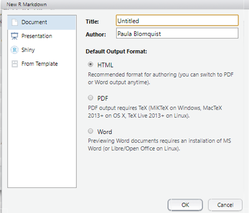
In RStudio, open a new R markdown file, starting with ‘File’, then ‘New file’ then ‘R markdown…’.
R Studio will give you some output options to pick from. In the example below we select “HTML” because we want to create an html document. The title and the author names are not important. If the output document type you want is not one of these, don’t worry - you can just pick any one and change it in the script later.
This will open up a new .Rmd script.
Important to know
The working directory
The working directory of a markdown file is wherever the Rmd file itself is saved. For instance, if the R project is within ~/Documents/projectX and the Rmd file itself is in a subfolder ~/Documents/projectX/markdownfiles/markdown.Rmd, the code read.csv(“data.csv”) within the markdown will look for a csv file in the markdownfiles folder, and not the root project folder where scripts within projects would normally automatically look.
To refer to files elsewhere, you will either need to use the full file path or use the here package. The here package sets the working directory to the root folder of the R project and is explained in detail in the R projects and Import and export pages of this handbook. For instance, to import a file called “data.csv” from within the projectX folder, the code would be import(here(“data.csv”)).
Note that use of setwd() in R Markdown scripts is not recommended – it only applies to the code chunk that it is written in.
Working on a drive vs your computer
Because R Markdown can run into pandoc issues when running on a shared network drive, it is recommended that your folder is on your local machine, e.g. in a project within ‘My Documents’. If you use Git (much recommended!), this will be familiar. For more details, see the handbook pages on R on network drives and Errors and help.
40.3 R Markdown components
An R Markdown document can be edited in RStudio just like a standard R script. When you start a new R Markdown script, RStudio tries to be helpful by showing a template which explains the different section of an R Markdown script.
The below is what appears when starting a new Rmd script intended to produce an html output (as per previous section).
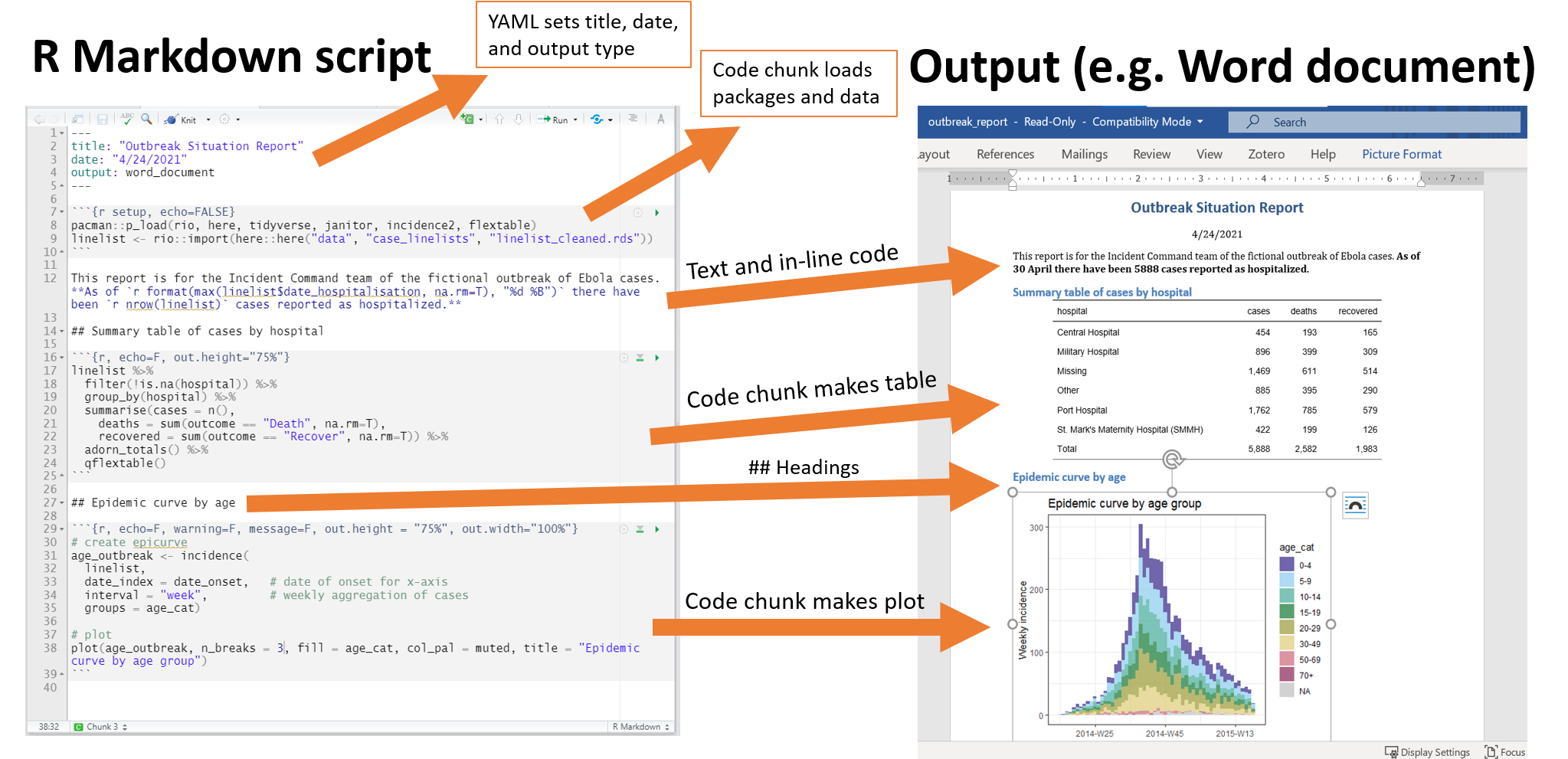
As you can see, there are three basic components to an Rmd file: YAML, Markdown text, and R code chunks.
These will create and become your document output. See the diagram below:
YAML metadata
Referred to as the ‘YAML metadata’ or just ‘YAML’, this is at the top of the R Markdown document. This section of the script will tell your Rmd file what type of output to produce, formatting preferences, and other metadata such as document title, author, and date. There are other uses not mentioned here (but referred to in ‘Producing an output’). Note that indentation matters; tabs are not accepted but spaces are.
This section must begin with a line containing just three dashes --- and must close with a line containing just three dashes ---. YAML parameters comes in key:value pairs. The placement of colons in YAML is important - the key:value pairs are separated by colons (not equals signs!).
The YAML should begin with metadata for the document. The order of these primary YAML parameters (not indented) does not matter. For example:
title: "My document"
author: "Me"
date: "2024-06-19"
You can use R code in YAML values by writing it as in-line code (preceded by r within back-ticks) but also within quotes (see above example for date:).
In the image above, because we clicked that our default output would be an html file, we can see that the YAML says output: html_document. However we can also change this to say powerpoint_presentation or word_document or even pdf_document.
Text
This is the narrative of your document, including the titles and headings. It is written in the “markdown” language, which is used across many different software.
Below are the core ways to write this text. See more extensive documentation available on R Markdown “cheatsheet” at the RStudio website.
New lines
Uniquely in R Markdown, to initiate a new line, enter *two spaces** at the end of the previous line and then Enter/Return.
Case
Surround your normal text with these character to change how it appears in the output.
- Underscores (
_text_) or single asterisk (*text*) to italicise - Double asterisks (
**text**) for bold text - Back-ticks (
text) to display text as code
The actual appearance of the font can be set by using specific templates (specified in the YAML metadata; see example tabs).
Color
There is no simple mechanism to change the color of text in R Markdown. One work-around, IF your output is an HTML file, is to add an HTML line into the markdown text. The below HTML code will print a line of text in bold red.
<span style="color: red;">**_DANGER:_** This is a warning.</span> DANGER: This is a warning.
Titles and headings
A hash symbol in a text portion of a R Markdown script creates a heading. This is different than in a chunk of R code in the script, in which a hash symbol is a mechanism to comment/annotate/de-activate, as in a normal R script.
Different heading levels are established with different numbers of hash symbols at the start of a new line. One hash symbol is a title or primary heading. Two hash symbols are a second-level heading. Third- and fourth-level headings can be made with successively more hash symbols.
# First-level heading / title

## Second level heading

### Third-level heading
Bullets and numbering
Use asterisks (*) to created a bullets list. Finish the previous sentence, enter two spaces, Enter/Return twice, and then start your bullets. Include a space between the asterisk and your bullet text. After each bullet enter two spaces and then Enter/Return. Sub-bullets work the same way but are indented. Numbers work the same way but instead of an asterisk, write 1), 2), etc. Below is how your R Markdown script text might look.
Here are my bullets (there are two spaces after this colon):

* Bullet 1 (followed by two spaces and Enter/Return)
* Bullet 2 (followed by two spaces and Enter/Return)
  * Sub-bullet 1 (followed by two spaces and Enter/Return)
  * Sub-bullet 2 (followed by two spaces and Enter/Return)
Code chunks
Sections of the script that are dedicated to running R code are called “chunks”. This is where you may load packages, import data, and perform the actual data management and visualisation. There may be many code chunks, so they can help you organize your R code into parts, perhaps interspersed with text. To note: These ‘chunks’ will appear to have a slightly different background colour from the narrative part of the document.
Each chunk is opened with a line that starts with three back-ticks, and curly brackets that contain parameters for the chunk ({ }). The chunk ends with three more back-ticks.
You can create a new chunk by typing it out yourself, by using the keyboard shortcut “Ctrl + Alt + i” (or Cmd + Shift + r in Mac), or by clicking the green ‘insert a new code chunk’ icon at the top of your script editor.
Some notes about the contents of the curly brackets { }:
- They start with ‘r’ to indicate that the language name within the chunk is R
- After the r you can optionally write a chunk “name” – these are not necessary but can help you organise your work. Note that if you name your chunks, you should ALWAYS use unique names or else R will complain when you try to render.
- The curly brackets can include other options too, written as
tag=value, such as:
eval = FALSEto not run the R code
echo = FALSEto not print the chunk’s R source code in the output document
warning = FALSEto not print warnings produced by the R code
message = FALSEto not print any messages produced by the R code
include =either TRUE/FALSE whether to include chunk outputs (e.g. plots) in the documentout.width =andout.height =- provide in styleout.width = "75%"
fig.align = "center"adjust how a figure is aligned across the page
fig.show='hold'if your chunk prints multiple figures and you want them printed next to each other (pair without.width = c("33%", "67%"). Can also set asfig.show='asis'to show them below the code that generates them,'hide'to hide, or'animate'to concatenate multiple into an animation.
- A chunk header must be written in one line
- Try to avoid periods, underscores, and spaces. Use hyphens ( - ) instead if you need a separator.
Read more extensively about the knitr options here.
Some of the above options can be configured with point-and-click using the setting buttons at the top right of the chunk. Here, you can specify which parts of the chunk you want the rendered document to include, namely the code, the outputs, and the warnings. This will come out as written preferences within the curly brackets, e.g. echo=FALSE if you specify you want to ‘Show output only’.
There are also two arrows at the top right of each chunk, which are useful to run code within a chunk, or all code in prior chunks. Hover over them to see what they do.
For global options to be applied to all chunks in the script, you can set this up within your very first R code chunk in the script. For instance, so that only the outputs are shown for each code chunk and not the code itself, you can include this command in the R code chunk:
knitr::opts_chunk$set(echo = FALSE) In-text R code
You can also include minimal R code within back-ticks. Within the back-ticks, begin the code with “r” and a space, so RStudio knows to evaluate the code as R code. See the example below.
The example below shows multiple heading levels, bullets, and uses R code for the current date (Sys.Date()) to evaluate into a printed date.
The example above is simple (showing the current date), but using the same syntax you can display values produced by more complex R code (e.g. to calculate the min, median, max of a column). You can also integrate R objects or values that were created in R code chunks earlier in the script.
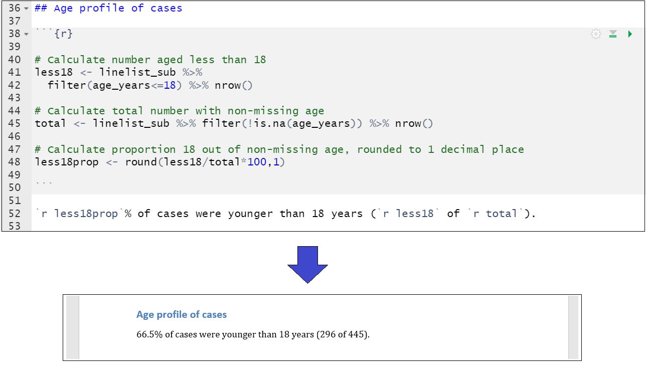
As an example, the script below calculates the proportion of cases that are aged less than 18 years old, using tidyverse functions, and creates the objects less18, total, and less18prop. This dynamic value is inserted into subsequent text. We see how it looks when knitted to a word document.
Images
You can include images in your R Markdown one of two ways:
 If the above does not work, try using knitr::include_graphics()
knitr::include_graphics("path/to/image.png")(remember, your file path could be written using the here package)
knitr::include_graphics(here::here("path", "to", "image.png"))Tables
Create a table using hyphens ( - ) and bars ( | ). The number of hyphens before/between bars allow the number of spaces in the cell before the text begins to wrap.
Column 1 |Column  2 |Column 3
---------|----------|--------
Cell A   |Cell B    |Cell C
Cell D   |Cell E    |Cell F
The above code produces the table below:
| Column 1 | Column 2 | Column 3 |
|---|---|---|
| Cell A | Cell B | Cell C |
| Cell D | Cell E | Cell F |
Tabbed sections
For HTML outputs, you can arrange the sections into “tabs”. Simply add .tabset in the curly brackets { } that are placed after a heading. Any sub-headings beneath that heading (until another heading of the same level) will appear as tabs that the user can click through. Read more here
You can add an additional option .tabset-pills after .tabset to give the tabs themselves a “pilled” appearance. Be aware that when viewing the tabbed HTML output, the Ctrl+f search functionality will only search “active” tabs, not hidden tabs.
40.4 File structure
There are several ways to structure your R Markdown and any associated R scripts. Each has advantages and disadvantages:
- Self-contained R Markdown - everything needed for the report is imported or created within the R Markdown
- Source other files - You can run external R scripts with the
source()command and use their outputs in the Rmd
- Child scripts - an alternate mechanism for
source()
- Source other files - You can run external R scripts with the
- Utilize a “runfile” - Run commands in an R script prior to rendering the R Markdown
Self-contained Rmd
For a relatively simple report, you may elect to organize your R Markdown script such that it is “self-contained” and does not involve any external scripts.
Everything you need to run the R markdown is imported or created within the Rmd file, including all the code chunks and package loading. This “self-contained” approach is appropriate when you do not need to do much data processing (e.g. it brings in a clean or semi-clean data file) and the rendering of the R Markdown will not take too long.
In this scenario, one logical organization of the R Markdown script might be:
- Set global knitr options
- Load packages
- Import data
- Process data
- Produce outputs (tables, plots, etc.)
- Save outputs, if applicable (.csv, .png, etc.)
Source other files
One variation of the “self-contained” approach is to have R Markdown code chunks “source” (run) other R scripts. This can make your R Markdown script less cluttered, more simple, and easier to organize. It can also help if you want to display final figures at the beginning of the report. In this approach, the final R Markdown script simply combines pre-processed outputs into a document.
One way to do this is by providing the R scripts (file path and name with extension) to the base R command source().
source("your-script.R", local = knitr::knit_global())
# or sys.source("your-script.R", envir = knitr::knit_global())
Note that when using source() within the R Markdown, the external files will still be run during the course of rendering your Rmd file. Therefore, each script is run every time you render the report. Thus, having these source() commands within the R Markdown does not speed up your run time, nor does it greatly assist with de-bugging, as error produced will still be printed when producing the R Markdown.
An alternative is to utilize the child = knitr option. EXPLAIN MORE TO DO
You must be aware of various R environments. Objects created within an environment will not necessarily be available to the environment used by the R Markdown.
Runfile
This approach involves utilizing the R script that contains the render() command(s) to pre-process objects that feed into the R markdown.
For instance, you can load the packages, load and clean the data, and even create the graphs of interest prior to render(). These steps can occur in the R script, or in other scripts that are sourced. As long as these commands occur in the same RStudio session and objects are saved to the environment, the objects can then be called within the Rmd content. Then the R markdown itself will only be used for the final step - to produce the output with all the pre-processed objects. This is much easier to de-bug if something goes wrong.
This approach is helpful for the following reasons:
- More informative error messages - these messages will be generated from the R script, not the R Markdown. R Markdown errors tend to tell you which chunk had a problem, but will not tell you which line.
- If applicable, you can run long processing steps in advance of the
render()command - they will run only once.
In the example below, we have a separate R script in which we pre-process a data object into the R Environment and then render the “create_output.Rmd” using render().
data <- import("datafile.csv") %>%       # Load data and save to environment
  select(age, hospital, weight)          # Select limited columns

rmarkdown::render(input = "create_output.Rmd")   # Create Rmd file
Folder strucutre
Workflow also concerns the overall folder structure, such as having an ‘output’ folder for created documents and figures, and ‘data’ or ‘inputs’ folders for cleaned data. We do not go into further detail here, but check out the Organizing routine reports page.
40.5 Producing the document
You can produce the document in the following ways:
- Manually by pressing the “Knit” button at the top of the RStudio script editor (fast and easy)
- Run the
render()command (executed outside the R Markdown script)
Option 2: render() command
Another way to produce your R Markdown output is to run the render() function (from the rmarkdown package). You must execute this command outside the R Markdown script - so either in a separate R script (often called a “run file”), or as a stand-alone command in the R Console.
rmarkdown::render(input = "my_report.Rmd")As with “knit”, the default settings will save the Rmd output to the same folder as the Rmd script, with the same file name (aside from the file extension). For instance “my_report.Rmd” when knitted will create “my_report.docx” if you are knitting to a word document. However, by using render() you have the option to use different settings. render() can accept arguments including:
output_format =This is the output format to convert to (e.g."html_document","pdf_document","word_document", or"all"). You can also specify this in the YAML inside the R Markdown script.
output_file =This is the name of the output file (and file path). This can be created via R functions likehere()orstr_glue()as demonstrated below.
output_dir =This is an output directory (folder) to save the file. This allows you to chose an alternative other than the directory the Rmd file is saved to.
output_options =You can provide a list of options that will override those in the script YAML (e.g. )output_yaml =You can provide path to a .yml file that contains YAML specifications
params =See the section on parameters below
- See the complete list here
As one example, to improve version control, the following command will save the output file within an ‘outputs’ sub-folder, with the current date in the file name. To create the file name, the function str_glue() from the stringr package is use to ‘glue’ together static strings (written plainly) with dynamic R code (written in curly brackets). For instance if it is April 10th 2021, the file name from below will be “Report_2021-04-10.docx”. See the page on Characters and strings for more details on str_glue().
rmarkdown::render(
  input = "create_output.Rmd",
  output_file = stringr::str_glue("outputs/Report_{Sys.Date()}.docx"))
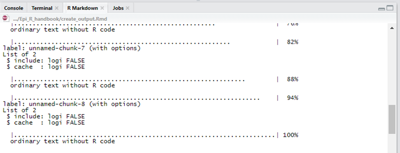
As the file renders, the RStudio Console will show you the rendering progress up to 100%, and a final message to indicate that the rendering is complete.
Options 3: reportfactory package
The R package reportfactory offers an alternative method of organising and compiling R Markdown reports catered to scenarios where you run reports routinely (e.g. daily, weekly…). It eases the compilation of multiple R Markdown files and the organization of their outputs. In essence, it provides a “factory” from which you can run the R Markdown reports, get automatically date- and time-stamped folders for the outputs, and have “light” version control.
Read more about this work flow in the page on Organizing routine reports.
40.6 Parameterised reports
You can use parameterisation to make a report dynamic, such that it can be run with specific setting (e.g. a specific date or place or with certain knitting options). Below, we focus on the basics, but there is more detail online about parameterized reports.
Using the Ebola linelist as an example, let’s say we want to run a standard surveillance report for each hospital each day. We show how one can do this using parameters.
Important: dynamic reports are also possible without the formal parameter structure (without params:), using simple R objects in an adjacent R script. This is explained at the end of this section.
Setting parameters
You have several options for specifying parameter values for your R Markdown output.
Option 1: Set parameters within YAML
Edit the YAML to include a params: option, with indented statements for each parameter you want to define. In this example we create parameters date and hospital, for which we specify values. These values are subject to change each time the report is run. If you use the “Knit” button to produce the output, the parameters will have these default values. Likewise, if you use render() the parameters will have these default values unless otherwise specified in the render() command.
---
title: Surveillance report
output: html_document
params:
 date: 2021-04-10
 hospital: Central Hospital
---
In the background, these parameter values are contained within a read-only list called params. Thus, you can insert the parameter values in R code as you would another R object/value in your environment. Simply type params$ followed by the parameter name. For example params$hospital to represent the hospital name (“Central Hospital” by default).
Note that parameters can also hold values true or false, and so these can be included in your knitr options for a R chunk. For example, you can set {r, eval=params$run} instead of {r, eval=FALSE}, and now whether the chunk runs or not depends on the value of a parameter run:.
Note that for parameters that are dates, they will be input as a string. So for params$date to be interpreted in R code it will likely need to be wrapped with as.Date() or a similar function to convert to class Date.
Option 2: Set parameters within render()
As mentioned above, as alternative to pressing the “Knit” button to produce the output is to execute the render() function from a separate script. In this later case, you can specify the parameters to be used in that rendering to the params = argument of render().
Note than any parameter values provided here will overwrite their default values if written within the YAML. We write the values in quotation marks as in this case they should be defined as character/string values.
The below command renders “surveillance_report.Rmd”, specifies a dynamic output file name and folder, and provides a list() of two parameters and their values to the argument params =.
rmarkdown::render(
  input = "surveillance_report.Rmd",
  output_file = stringr::str_glue("outputs/Report_{Sys.Date()}.docx"),
  params = list(date = "2021-04-10", hospital  = "Central Hospital"))
Option 3: Set parameters using a Graphical User Interface
For a more interactive feel, you can also use the Graphical User Interface (GUI) to manually select values for parameters. To do this we can click the drop-down menu next to the ‘Knit’ button and choose ‘Knit with parameters’.
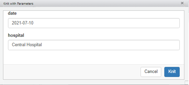
A pop-up will appear allowing you to type in values for the parameters that are established in the document’s YAML.
You can achieve the same through a render() command by specifying params = "ask", as demonstrated below.
rmarkdown::render(
  input = "surveillance_report.Rmd",
  output_file = stringr::str_glue("outputs/Report_{Sys.Date()}.docx"),
  params = “ask”)
However, typing values into this pop-up window is subject to error and spelling mistakes. You may prefer to add restrictions to the values that can be entered through drop-down menus. You can do this by adding in the YAML several specifications for each params: entry.
label:is how the title for that particular drop-down menu
value:is the default (starting) value
input:set toselectfor drop-down menu
choices:Give the eligible values in the drop-down menu
Below, these specifications are written for the hospital parameter.
---
title: Surveillance report
output: html_document
params:
 date: 2021-04-10
 hospital:
  label: “Town:”
  value: Central Hospital
  input: select
  choices: [Central Hospital, Military Hospital, Port Hospital, St. Mark's Maternity Hospital (SMMH)]
---
When knitting (either via the ‘knit with parameters’ button or by render()), the pop-up window will have drop-down options to select from.
Parameterized example
The following code creates parameters for date and hospital, which are used in the R Markdown as params$date and params$hospital, respectively.
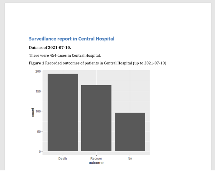
In the resulting report output, see how the data are filtered to the specific hospital, and the plot title refers to the correct hospital and date. We use the “linelist_cleaned.rds” file here, but it would be particularly appropriate if the linelist itself also had a datestamp within it to align with parameterised date.
Knitting this produces the final output with the default font and layout.
Parameterisation without params
If you are rendering a R Markdown file with render() from a separate script, you can actually create the impact of parameterization without using the params: functionality.
For instance, in the R script that contains the render() command, you can simply define hospital and date as two R objects (values) before the render() command. In the R Markdown, you would not need to have a params: section in the YAML, and we would refer to the date object rather than params$date and hospital rather than params$hospital.
# This is a R script that is separate from the R Markdown

# define R objects
hospital <- "Central Hospital"
date <- "2021-04-10"

# Render the R markdown
rmarkdown::render(input = "create_output.Rmd")
Following this approach means means you can not “knit with parameters”, use the GUI, or include knitting options within the parameters. However it allows for simpler code, which may be advantageous.
40.7 Looping reports
We may want to run a report multiple times, varying the input parameters, to produce a report for each jurisdictions/unit. This can be done using tools for iteration, which are explained in detail in the page on Iteration, loops, and lists. Options include the purrr package, or use of a for loop as explained below.
Below, we use a simple for loop to generate a surveillance report for all hospitals of interest. This is done with one command (instead of manually changing the hospital parameter one-at-a-time). The command to render the reports must exist in a separate script outside the report Rmd. This script will also contain defined objects to “loop through” - today’s date, and a vector of hospital names to loop through.
hospitals <- c("Central Hospital",
                "Military Hospital",
                "Port Hospital",
                "St. Mark's Maternity Hospital (SMMH)")
We then feed these values one-at-a-time into the render() command using a loop, which runs the command once for each value in the hospitals vector. The letter i represents the index position (1 through 4) of the hospital currently being used in that iteration, such that hospital_list[1] would be “Central Hospital”. This information is supplied in two places in the render() command:
- To the file name, such that the file name of the first iteration if produced on 10th April 2021 would be “Report_Central Hospital_2021-04-10.docx”, saved in the ‘output’ subfolder of the working directory.
- To
params =such that the Rmd uses the hospital name internally whenever theparams$hospitalvalue is called (e.g. to filter the dataset to the particular hospital only). In this example, four files would be created - one for each hospital.
for(i in 1:length(hospitals)){
  rmarkdown::render(
    input = "surveillance_report.Rmd",
    output_file = str_glue("output/Report_{hospitals[i]}_{Sys.Date()}.docx"),
    params = list(hospital  = hospitals[i]))
}
40.8 Templates
By using a template document that contains any desired formatting, you can adjust the aesthetics of how the Rmd output will look. You can create for instance an MS Word or Powerpoint file that contains pages/slides with the desired dimensions, watermarks, backgrounds, and fonts.
Word documents
To create a template, start a new word document (or use an existing output with formatting the suits you), and edit fonts by defining the Styles. In Style,Headings 1, 2, and 3 refer to the various markdown header levels (# Header 1, ## Header 2 and ### Header 3 respectively). Right click on the style and click ‘modify’ to change the font formatting as well as the paragraph (e.g. you can introduce page breaks before certain styles which can help with spacing). Other aspects of the word document such as margins, page size, headers etc, can be changed like a usual word document you are working directly within.
Powerpoint documents
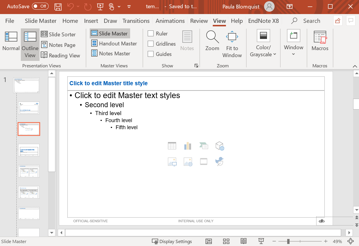
As above, create a new slideset or use an existing powerpoint file with the desired formatting. For further editing, click on ‘View’ and ‘Slide Master’. From here you can change the ‘master’ slide appearance by editing the text formatting in the text boxes, as well as the background/page dimensions for the overall page.
Unfortunately, editing powerpoint files is slightly less flexible:
- A first level header (
# Header 1) will automatically become the title of a new slide, - A
## Header 2text will not come up as a subtitle but text within the slide’s main textbox (unless you find a way to maniuplate the Master view). - Outputted plots and tables will automatically go into new slides. You will need to combine them, for instance the the patchwork function to combine ggplots, so that they show up on the same page. See this blog post about using the patchwork package to put multiple images on one slide.
See the officer package for a tool to work more in-depth with powerpoint presentations.
Integrating templates into the YAML
Once a template is prepared, the detail of this can be added in the YAML of the Rmd underneath the ‘output’ line and underneath where the document type is specified (which goes to a separate line itself). Note reference_doc can be used for powerpoint slide templates.
It is easiest to save the template in the same folder as where the Rmd file is (as in the example below), or in a subfolder within.
---
title: Surveillance report
output:
 word_document:
  reference_docx: "template.docx"
params:
 date: 2021-04-10
 hospital: Central Hospital
template:

---
Formatting HTML files
HTML files do not use templates, but can have the styles configured within the YAML. HTMLs are interactive documents, and are particularly flexible. We cover some basic options here.
Table of contents: We can add a table of contents with
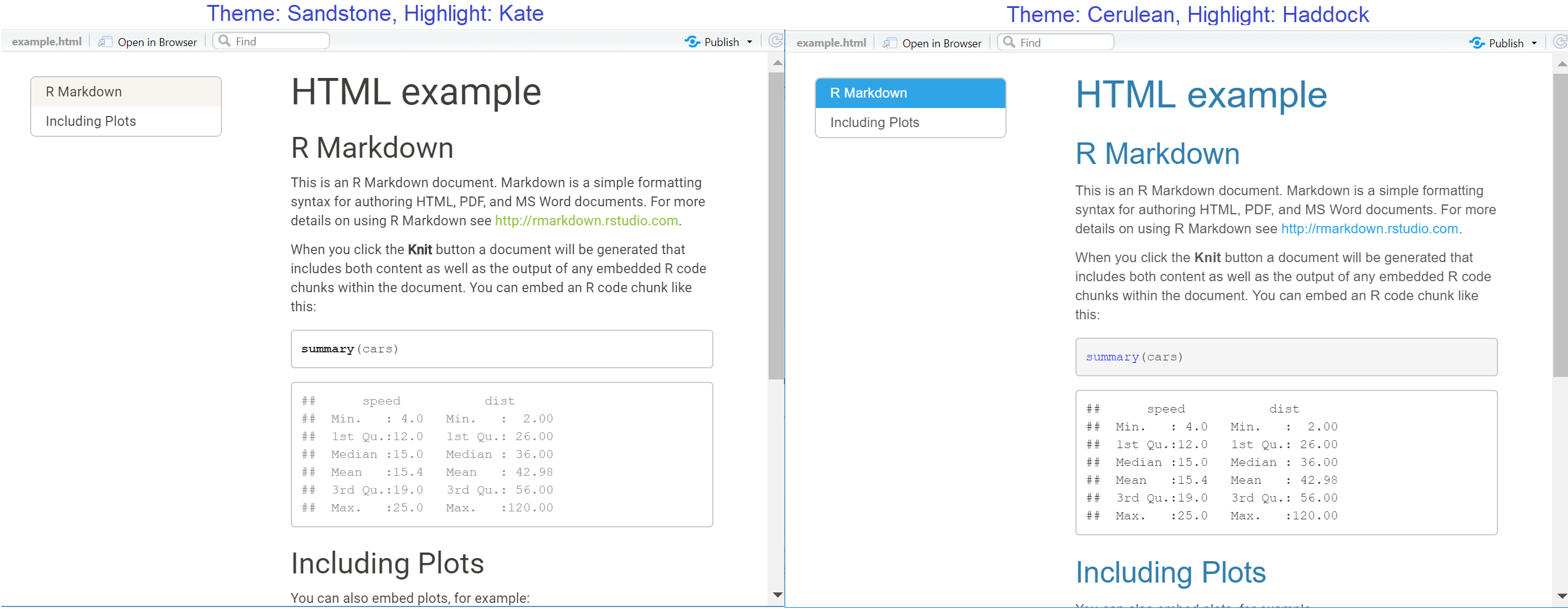
toc: truebelow, and also specify that it remains viewable (“floats”) as you scroll, withtoc_float: true.Themes: We can refer to some pre-made themes, which come from a Bootswatch theme library. In the below example we use cerulean. Other options include: journal, flatly, darkly, readable, spacelab, united, cosmo, lumen, paper, sandstone, simplex, and yeti.
Highlight: Configuring this changes the look of highlighted text (e.g. code within chunks that are shown). Supported styles include default, tango, pygments, kate, monochrome, espresso, zenburn, haddock, breezedark, and textmate.
Here is an example of how to integrate the above options into the YAML.
---
title: "HTML example"
output:
  html_document:
    toc: true
    toc_float: true
    theme: cerulean
    highlight: kate

---
Below are two examples of HTML outputs which both have floating tables of contents, but different theme and highlight styles selected:
40.9 Dynamic content
In an HTML output, your report content can be dynamic. Below are some examples:
Tables
In an HTML report, you can print data frame / tibbles such that the content is dynamic, with filters and scroll bars. There are several packages that offer this capability.
To do this with the DT package, as is used throughout this handbook, you can insert a code chunk like this:
The function datatable() will print the provided data frame as a dynamic table for the reader. You can set rownames = FALSE to simplify the far left-side of the table. filter = "top" provides a filter over each column. In the option() argument provide a list of other specifications. Below we include two: pageLength = 5 set the number of rows that appear as 5 (the remaining rows can be viewed by paging through arrows), and scrollX=TRUE enables a scrollbar on the bottom of the table (for columns that extend too far to the right).
If your dataset is very large, consider only showing the top X rows by wrapping the data frame in head().
HTML widgets
HTML widgets for R are a special class of R packages that enable increased interactivity by utilizing JavaScript libraries. You can embed them in HTML R Markdown outputs.
Some common examples of these widgets include:
- Plotly (used in this handbook page and in the Interative plots page)
- visNetwork (used in the Transmission Chains page of this handbook)
- Leaflet (used in the GIS Basics page of this handbook)
- dygraphs (useful for interactively showing time series data)
- DT (
datatable()) (used to show dynamic tables with filter, sort, etc.)
The ggplotly() function from plotly is particularly easy to use. See the Interactive plots page.
40.10 Resources
Further information can be found via:
- https://bookdown.org/yihui/rmarkdown/
- https://rmarkdown.rstudio.com/articles_intro.html
A good explainer of markdown vs knitr vs Rmarkdown is here: https://stackoverflow.com/questions/40563479/relationship-between-r-markdown-knitr-pandoc-and-bookdown











Comment out text
You can “comment out” R Markdown text just as you can use the “#” to comment out a line of R code in an R chunk. Simply highlight the text and press Ctrl+Shift+c (Cmd+Shift+c for Mac). The text will be surrounded by arrows and turn green. It will not appear in your output.