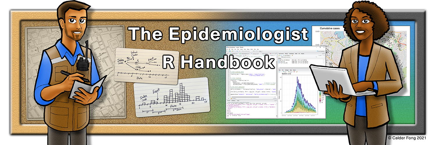
× Need help learning R? Enroll in Applied Epi's intro R course, try our free R tutorials, post in our Community Q&A forum, or ask about our R Help Desk service.

7 Import and export

In this page we describe ways to locate, import, and export files:

  • Use of the rio package to flexibly import() and export() many types of files
  • Use of the here package to locate files relative to an R project root - to prevent complications from file paths that are specific to one computer
  • Specific import scenarios, such as:
    • Specific Excel sheets
    • Messy headers and skipping rows
    • From Google sheets
    • From data posted to websites
    • With APIs
    • Importing the most recent file
  • Manual data entry
  • R-specific file types such as RDS and RData
  • Exporting/saving files and plots

7.1 Overview

When you import a “dataset” into R, you are generally creating a new data frame object in your R environment and defining it as an imported file (e.g. Excel, CSV, TSV, RDS) that is located in your folder directories at a certain file path/address.

You can import/export many types of files, including those created by other statistical programs (SAS, STATA, SPSS). You can also connect to relational databases.

R even has its own data formats:

  • An RDS file (.rds) stores a single R object such as a data frame. These are useful to store cleaned data, as they maintain R column classes. Read more in this section.
  • An RData file (.Rdata) can be used to store multiple objects, or even a complete R workspace. Read more in this section.

7.2 The rio package

The R package we recommend is: rio. The name “rio” is an abbreviation of “R I/O” (input/output).

Its functions import() and export() can handle many different file types (e.g. .xlsx, .csv, .rds, .tsv). When you provide a file path to either of these functions (including the file extension like “.csv”), rio will read the extension and use the correct tool to import or export the file.

The alternative to using rio is to use functions from many other packages, each of which is specific to a type of file. For example, read.csv() (base R), read.xlsx() (openxlsx package), and write_csv() (readr pacakge), etc. These alternatives can be difficult to remember, whereas using import() and export() from rio is easy.

rio’s functions import() and export() use the appropriate package and function for a given file, based on its file extension. See the end of this page for a complete table of which packages/functions rio uses in the background. It can also be used to import STATA, SAS, and SPSS files, among dozens of other file types.

Import/export of shapefiles requires other packages, as detailed in the page on GIS basics.

7.3 The here package

The package here and its function here() make it easy to tell R where to find and to save your files - in essence, it builds file paths.

Used in conjunction with an R project, here allows you to describe the location of files in your R project in relation to the R project’s root directory (the top-level folder). This is useful when the R project may be shared or accessed by multiple people/computers. It prevents complications due to the unique file paths on different computers (e.g. "C:/Users/Laura/Documents..." by “starting” the file path in a place common to all users (the R project root).

This is how here() works within an R project:

  • When the here package is first loaded within the R project, it places a small file called “.here” in the root folder of your R project as a “benchmark” or “anchor”
  • In your scripts, to reference a file in the R project’s sub-folders, you use the function here() to build the file path in relation to that anchor
  • To build the file path, write the names of folders beyond the root, within quotes, separated by commas, finally ending with the file name and file extension as shown below
  • here() file paths can be used for both importing and exporting

For example, below, the function import() is being provided a file path constructed with here().

linelist <- import(here("data", "linelists", "ebola_linelist.xlsx"))

The command here("data", "linelists", "ebola_linelist.xlsx") is actually providing the full file path that is unique to the user’s computer:

"C:/Users/Laura/Documents/my_R_project/data/linelists/ebola_linelist.xlsx"

The beauty is that the R command using here() can be successfully run on any computer accessing the R project.

TIP: If you are unsure where the “.here” root is set to, run the function here() with empty parentheses.

Read more about the here package at this link.

7.4 File paths

When importing or exporting data, you must provide a file path. You can do this one of three ways:

  1. Recommended: provide a “relative” file path with the here package
  2. Provide the “full” / “absolute” file path
  3. Manual file selection

“Relative” file paths

In R, “relative” file paths consist of the file path relative to the root of an R project. They allow for more simple file paths that can work on different computers (e.g. if the R project is on a shared drive or is sent by email). As described above, relative file paths are facilitated by use of the here package.

An example of a relative file path constructed with here() is below. We assume the work is in an R project that contains a sub-folder “data” and within that a subfolder “linelists”, in which there is the .xlsx file of interest.

linelist <- import(here("data", "linelists", "ebola_linelist.xlsx"))

“Absolute” file paths

Absolute or “full” file paths can be provided to functions like import() but they are “fragile” as they are unique to the user’s specific computer and therefore not recommended.

Below is an example of an absolute file path, where in Laura’s computer there is a folder “analysis”, a sub-folder “data” and within that a sub-folder “linelists”, in which there is the .xlsx file of interest.

linelist <- import("C:/Users/Laura/Documents/analysis/data/linelists/ebola_linelist.xlsx")

A few things to note about absolute file paths:

  • Avoid using absolute file paths as they will break if the script is run on a different computer
  • Use forward slashes (/), as in the example above (note: this is NOT the default for Windows file paths)
  • File paths that begin with double slashes (e.g. “//…”) will likely not be recognized by R and will produce an error. Consider moving your work to a “named” or “lettered” drive that begins with a letter (e.g. “J:” or “C:”). See the page on Directory interactions for more details on this issue.

One scenario where absolute file paths may be appropriate is when you want to import a file from a shared drive that has the same full file path for all users.

TIP: To quickly convert all \ to /, highlight the code of interest, use Ctrl+f (in Windows), check the option box for “In selection”, and then use the replace functionality to convert them.

Select file manually

You can import data manually via one of these methods:

  1. Environment RStudio Pane, click “Import Dataset”, and select the type of data
  2. Click File / Import Dataset / (select the type of data)
  3. To hard-code manual selection, use the base R command file.choose() (leaving the parentheses empty) to trigger appearance of a pop-up window that allows the user to manually select the file from their computer. For example:
# Manual selection of a file. When this command is run, a POP-UP window will appear. 
# The file path selected will be supplied to the import() command.

my_data <- import(file.choose())

TIP: The pop-up window may appear BEHIND your RStudio window.

7.5 Import data

To use import() to import a dataset is quite simple. Simply provide the path to the file (including the file name and file extension) in quotes. If using here() to build the file path, follow the instructions above. Below are a few examples:

Importing a csv file that is located in your “working directory” or in the R project root folder:

linelist <- import("linelist_cleaned.csv")

Importing the first sheet of an Excel workbook that is located in “data” and “linelists” sub-folders of the R project (the file path built using here()):

linelist <- import(here("data", "linelists", "linelist_cleaned.xlsx"))

Importing a data frame (a .rds file) using an absolute file path:

linelist <- import("C:/Users/Laura/Documents/tuberculosis/data/linelists/linelist_cleaned.rds")

Specific Excel sheets

By default, if you provide an Excel workbook (.xlsx) to import(), the workbook’s first sheet will be imported. If you want to import a specific sheet, include the sheet name to the which = argument. For example:

my_data <- import("my_excel_file.xlsx", which = "Sheetname")

If using the here() method to provide a relative pathway to import(), you can still indicate a specific sheet by adding the which = argument after the closing parentheses of the here() function.

# Demonstration: importing a specific Excel sheet when using relative pathways with the 'here' package
linelist_raw <- import(here("data", "linelist.xlsx"), which = "Sheet1")`  

To export a data frame from R to a specific Excel sheet and have the rest of the Excel workbook remain unchanged, you will have to import, edit, and export with an alternative package catered to this purpose such as openxlsx. See more information in the page on Directory interactions or at this github page.

If your Excel workbook is .xlsb (binary format Excel workbook) you may not be able to import it using rio. Consider re-saving it as .xlsx, or using a package like readxlsb which is built for this purpose.

Missing values

You may want to designate which value(s) in your dataset should be considered as missing. As explained in the page on Missing data, the value in R for missing data is NA, but perhaps the dataset you want to import uses 99, “Missing”, or just empty character space “” instead.

Use the na = argument for import() and provide the value(s) within quotes (even if they are numbers). You can specify multiple values by including them within a vector, using c() as shown below.

Here, the value “99” in the imported dataset is considered missing and converted to NA in R.

linelist <- import(here("data", "my_linelist.xlsx"), na = "99")

Here, any of the values “Missing”, “” (empty cell), or ” ” (single space) in the imported dataset are converted to NA in R.

linelist <- import(here("data", "my_linelist.csv"), na = c("Missing", "", " "))

Skip rows

Sometimes, you may want to avoid importing a row of data. You can do this with the argument skip = if using import() from rio on a .xlsx or .csv file. Provide the number of rows you want to skip.

linelist_raw <- import("linelist_raw.xlsx", skip = 1)  # does not import header row

Unfortunately skip = only accepts one integer value, not a range (e.g. “2:10” does not work). To skip import of specific rows that are not consecutive from the top, consider importing multiple times and using bind_rows() from dplyr. See the example below of skipping only row 2.

Manage a second header row

Sometimes, your data may have a second row, for example if it is a “data dictionary” row as shown below. This situation can be problematic because it can result in all columns being imported as class “character”.

Below is an example of this kind of dataset (with the first row being the data dictionary).

Remove the second header row

To drop the second header row, you will likely need to import the data twice.

  1. Import the data in order to store the correct column names
  2. Import the data again, skipping the first two rows (header and second rows)
  3. Bind the correct names onto the reduced dataframe

The exact argument used to bind the correct column names depends on the type of data file (.csv, .tsv, .xlsx, etc.). This is because rio is using a different function for the different file types (see table above).

For Excel files: (col_names =)

# import first time; store the column names
linelist_raw_names <- import("linelist_raw.xlsx") %>% names()  # save true column names

# import second time; skip row 2, and assign column names to argument col_names =
linelist_raw <- import("linelist_raw.xlsx",
                       skip = 2,
                       col_names = linelist_raw_names
                       ) 

For CSV files: (col.names =)

# import first time; sotre column names
linelist_raw_names <- import("linelist_raw.csv") %>% names() # save true column names

# note argument for csv files is 'col.names = '
linelist_raw <- import("linelist_raw.csv",
                       skip = 2,
                       col.names = linelist_raw_names
                       ) 

Backup option - changing column names as a separate command

# assign/overwrite headers using the base 'colnames()' function
colnames(linelist_raw) <- linelist_raw_names

Make a data dictionary

Bonus! If you do have a second row that is a data dictionary, you can easily create a proper data dictionary from it. This tip is adapted from this post.

dict <- linelist_2headers %>%             # begin: linelist with dictionary as first row
  head(1) %>%                             # keep only column names and first dictionary row                
  pivot_longer(cols = everything(),       # pivot all columns to long format
               names_to = "Column",       # assign new column names
               values_to = "Description")

Combine the two header rows

In some cases when your raw dataset has two header rows (or more specifically, the 2nd row of data is a secondary header), you may want to “combine” them or add the values in the second header row into the first header row.

The command below will define the data frame’s column names as the combination (pasting together) of the first (true) headers with the value immediately underneath (in the first row).

names(my_data) <- paste(names(my_data), my_data[1, ], sep = "_")

Google sheets

You can import data from an online Google spreadsheet with the googlesheet4 package and by authenticating your access to the spreadsheet.

pacman::p_load("googlesheets4")

Below, a demo Google sheet is imported and saved. This command may prompt confirmation of authentification of your Google account. Follow prompts and pop-ups in your internet browser to grant Tidyverse API packages permissions to edit, create, and delete your spreadsheets in Google Drive.

The sheet below is “viewable for anyone with the link” and you can try to import it.

Gsheets_demo <- read_sheet("https://docs.google.com/spreadsheets/d/1scgtzkVLLHAe5a6_eFQEwkZcc14yFUx1KgOMZ4AKUfY/edit#gid=0")

The sheet can also be imported using only the sheet ID, a shorter part of the URL:

Gsheets_demo <- read_sheet("1scgtzkVLLHAe5a6_eFQEwkZcc14yFUx1KgOMZ4AKUfY")

Another package, googledrive offers useful functions for writing, editing, and deleting Google sheets. For example, using the gs4_create() and sheet_write() functions found in this package.

Here are some other helpful online tutorials:
basic Google sheets importing tutorial
more detailed tutorial
interaction between the googlesheets4 and tidyverse

7.6 Multiple files - import, export, split, combine

See the page on Iteration, loops, and lists for examples of how to import and combine multiple files, or multiple Excel workbook files. That page also has examples on how to split a data frame into parts and export each one separately, or as named sheets in an Excel workbook.

7.7 Import from Github

Importing data directly from Github into R can be very easy or can require a few steps - depending on the file type. Below are some approaches:

CSV files

It can be easy to import a .csv file directly from Github into R with an R command.

  1. Go to the Github repo, locate the file of interest, and click on it
  2. Click on the “Raw” button (you will then see the “raw” csv data, as shown below)
  3. Copy the URL (web address)
  4. Place the URL in quotes within the import() R command

XLSX files

You may not be able to view the “Raw” data for some files (e.g. .xlsx, .rds, .nwk, .shp)

  1. Go to the Github repo, locate the file of interest, and click on it
  2. Click the “Download” button, as shown below
  3. Save the file on your computer, and import it into R

Shapefiles

Shapefiles have many sub-component files, each with a different file extention. One file will have the “.shp” extension, but others may have “.dbf”, “.prj”, etc. To download a shapefile from Github, you will need to download each of the sub-component files individually, and save them in the same folder on your computer. In Github, click on each file individually and download them by clicking on the “Download” button.

Once saved to your computer you can import the shapefile as shown in the GIS basics page using st_read() from the sf package. You only need to provide the filepath and name of the “.shp” file - as long as the other related files are within the same folder on your computer.

Below, you can see how the shapefile “sle_adm3” consists of many files - each of which must be downloaded from Github.

7.8 Manual data entry

Entry by rows

Use the tribble function from the tibble package from the tidyverse (online tibble reference).

Note how column headers start with a tilde (~). Also note that each column must contain only one class of data (character, numeric, etc.). You can use tabs, spacing, and new rows to make the data entry more intuitive and readable. Spaces do not matter between values, but each row is represented by a new line of code. For example:

# create the dataset manually by row
manual_entry_rows <- tibble::tribble(
  ~colA, ~colB,
  "a",   1,
  "b",   2,
  "c",   3
  )

And now we display the new dataset:

Entry by columns

Since a data frame consists of vectors (vertical columns), the base approach to manual dataframe creation in R expects you to define each column and then bind them together. This can be counter-intuitive in epidemiology, as we usually think about our data in rows (as above).

# define each vector (vertical column) separately, each with its own name
PatientID <- c(235, 452, 778, 111)
Treatment <- c("Yes", "No", "Yes", "Yes")
Death     <- c(1, 0, 1, 0)

CAUTION: All vectors must be the same length (same number of values).

The vectors can then be bound together using the function data.frame():

# combine the columns into a data frame, by referencing the vector names
manual_entry_cols <- data.frame(PatientID, Treatment, Death)

And now we display the new dataset:

Pasting from clipboard

If you copy data from elsewhere and have it on your clipboard, you can try one of the two ways below:

From the clipr package, you can use read_clip_tbl() to import as a data frame, or just just read_clip() to import as a character vector. In both cases, leave the parentheses empty.

linelist <- clipr::read_clip_tbl()  # imports current clipboard as data frame
linelist <- clipr::read_clip()      # imports as character vector

You can also easily export to your system’s clipboard with clipr. See the section below on Export.

Alternatively, you can use the the read.table() function from base R with file = "clipboard") to import as a data frame:

df_from_clipboard <- read.table(
  file = "clipboard",  # specify this as "clipboard"
  sep = "t",           # separator could be tab, or commas, etc.
  header=TRUE)         # if there is a header row

7.9 Import most recent file

Often you may receive daily updates to your datasets. In this case you will want to write code that imports the most recent file. Below we present two ways to approach this:

  • Selecting the file based on the date in the file name
  • Selecting the file based on file metadata (last modification)

Dates in file name

This approach depends on three premises:

  1. You trust the dates in the file names
  2. The dates are numeric and appear in generally the same format (e.g. year then month then day)
  3. There are no other numbers in the file name

We will explain each step, and then show you them combined at the end.

First, use dir() from base R to extract just the file names for each file in the folder of interest. See the page on Directory interactions for more details about dir(). In this example, the folder of interest is the folder “linelists” within the folder “example” within “data” within the R project.

linelist_filenames <- dir(here("data", "example", "linelists")) # get file names from folder
linelist_filenames                                              # print
## [1] "20201007linelist.csv"          "case_linelist_2020-10-02.csv"  "case_linelist_2020-10-03.csv" 
## [4] "case_linelist_2020-10-04.csv"  "case_linelist_2020-10-05.csv"  "case_linelist_2020-10-08.xlsx"
## [7] "case_linelist20201006.csv"

Once you have this vector of names, you can extract the dates from them by applying str_extract() from stringr using this regular expression. It extracts any numbers in the file name (including any other characters in the middle such as dashes or slashes). You can read more about stringr in the [Strings and characters] page.

linelist_dates_raw <- stringr::str_extract(linelist_filenames, "[0-9].*[0-9]") # extract numbers and any characters in between
linelist_dates_raw  # print
## [1] "20201007"   "2020-10-02" "2020-10-03" "2020-10-04" "2020-10-05" "2020-10-08" "20201006"

Assuming the dates are written in generally the same date format (e.g. Year then Month then Day) and the years are 4-digits, you can use lubridate’s flexible conversion functions (ymd(), dmy(), or mdy()) to convert them to dates. For these functions, the dashes, spaces, or slashes do not matter, only the order of the numbers. Read more in the Working with dates page.

linelist_dates_clean <- lubridate::ymd(linelist_dates_raw)
linelist_dates_clean
## [1] "2020-10-07" "2020-10-02" "2020-10-03" "2020-10-04" "2020-10-05" "2020-10-08" "2020-10-06"

The base R function which.max() can then be used to return the index position (e.g. 1st, 2nd, 3rd, …) of the maximum date value. The latest file is correctly identified as the 6th file - “case_linelist_2020-10-08.xlsx”.

index_latest_file <- which.max(linelist_dates_clean)
index_latest_file
## [1] 6

If we condense all these commands, the complete code could look like below. Note that the . in the last line is a placeholder for the piped object at that point in the pipe sequence. At that point the value is simply the number 6. This is placed in double brackets to extract the 6th element of the vector of file names produced by dir().

# load packages
pacman::p_load(
  tidyverse,         # data management
  stringr,           # work with strings/characters
  lubridate,         # work with dates
  rio,               # import / export
  here,              # relative file paths
  fs)                # directory interactions

# extract the file name of latest file
latest_file <- dir(here("data", "example", "linelists")) %>%  # file names from "linelists" sub-folder          
  str_extract("[0-9].*[0-9]") %>%                  # pull out dates (numbers)
  ymd() %>%                                        # convert numbers to dates (assuming year-month-day format)
  which.max() %>%                                  # get index of max date (latest file)
  dir(here("data", "example", "linelists"))[[.]]              # return the filename of latest linelist

latest_file  # print name of latest file
## [1] "case_linelist_2020-10-08.xlsx"

You can now use this name to finish the relative file path, with here():

here("data", "example", "linelists", latest_file) 

And you can now import the latest file:

# import
import(here("data", "example", "linelists", latest_file)) # import 

Use the file info

If your files do not have dates in their names (or you do not trust those dates), you can try to extract the last modification date from the file metadata. Use functions from the package fs to examine the metadata information for each file, which includes the last modification time and the file path.

Below, we provide the folder of interest to fs’s dir_info(). In this case, the folder of interest is in the R project in the folder “data”, the sub-folder “example”, and its sub-folder “linelists”. The result is a data frame with one line per file and columns for modification_time, path, etc. You can see a visual example of this in the page on Directory interactions.

We can sort this data frame of files by the column modification_time, and then keep only the top/latest row (file) with base R’s head(). Then we can extract the file path of this latest file only with the dplyr function pull() on the column path. Finally we can pass this file path to import(). The imported file is saved as latest_file.

latest_file <- dir_info(here("data", "example", "linelists")) %>%  # collect file info on all files in directory
  arrange(desc(modification_time)) %>%      # sort by modification time
  head(1) %>%                               # keep only the top (latest) file
  pull(path) %>%                            # extract only the file path
  import()                                  # import the file

7.10 APIs

An “Automated Programming Interface” (API) can be used to directly request data from a website. APIs are a set of rules that allow one software application to interact with another. The client (you) sends a “request” and receives a “response” containing content. The R packages httr and jsonlite can facilitate this process.

Each API-enabled website will have its own documentation and specifics to become familiar with. Some sites are publicly available and can be accessed by anyone. Others, such as platforms with user IDs and credentials, require authentication to access their data.

Needless to say, it is necessary to have an internet connection to import data via API. We will briefly give examples of use of APIs to import data, and link you to further resources.

Note: recall that data may be posted* on a website without an API, which may be easier to retrieve. For example a posted CSV file may be accessible simply by providing the site URL to import() as described in the section on importing from Github.*

HTTP request

The API exchange is most commonly done through an HTTP request. HTTP is Hypertext Transfer Protocol, and is the underlying format of a request/response between a client and a server. The exact input and output may vary depending on the type of API but the process is the same - a “Request” (often HTTP Request) from the user, often containing a query, followed by a “Response”, containing status information about the request and possibly the requested content.

Here are a few components of an HTTP request:

  • The URL of the API endpoint
  • The “Method” (or “Verb”)
  • Headers
  • Body

The HTTP request “method” is the action your want to perform. The two most common HTTP methods are GET and POST but others could include PUT, DELETE, PATCH, etc. When importing data into R it is most likely that you will use GET.

After your request, your computer will receive a “response” in a format similar to what you sent, including URL, HTTP status (Status 200 is what you want!), file type, size, and the desired content. You will then need to parse this response and turn it into a workable data frame within your R environment.

Packages

The httr package works well for handling HTTP requests in R. It requires little prior knowledge of Web APIs and can be used by people less familiar with software development terminology. In addition, if the HTTP response is .json, you can use jsonlite to parse the response.

# load packages
pacman::p_load(httr, jsonlite, tidyverse)

Publicly-available data

Below is an example of an HTTP request, borrowed from a tutorial from the Trafford Data Lab. This site has several other resources to learn and API exercises.

Scenario: We want to import a list of fast food outlets in the city of Trafford, UK. The data can be accessed from the API of the Food Standards Agency, which provides food hygiene rating data for the United Kingdom.

Here are the parameters for our request:

The R code would be as follows:

# prepare the request
path <- "http://api.ratings.food.gov.uk/Establishments"
request <- GET(url = path,
             query = list(
               localAuthorityId = 188,
               BusinessTypeId = 7844,
               pageNumber = 1,
               pageSize = 5000),
             add_headers("x-api-version" = "2"))

# check for any server error ("200" is good!)
request$status_code

# submit the request, parse the response, and convert to a data frame
response <- content(request, as = "text", encoding = "UTF-8") %>%
  fromJSON(flatten = TRUE) %>%
  pluck("establishments") %>%
  as_tibble()

You can now clean and use the response data frame, which contains one row per fast food facility.

Authentication required

Some APIs require authentication - for you to prove who you are, so you can access restricted data. To import these data, you may need to first use a POST method to provide a username, password, or code. This will return an access token, that can be used for subsequent GET method requests to retrieve the desired data.

Below is an example of querying data from Go.Data, which is an outbreak investigation tool. Go.Data uses an API for all interactions between the web front-end and smartphone applications used for data collection. Go.Data is used throughout the world. Because outbreak data are sensitive and you should only be able to access data for your outbreak, authentication is required.

Below is some sample R code using httr and jsonlite for connecting to the Go.Data API to import data on contact follow-up from your outbreak.

# set credentials for authorization
url <- "https://godatasampleURL.int/"           # valid Go.Data instance url
username <- "username"                          # valid Go.Data username 
password <- "password"                          # valid Go,Data password 
outbreak_id <- "xxxxxx-xxxx-xxxx-xxxx-xxxxxxx"  # valid Go.Data outbreak ID

# get access token
url_request <- paste0(url,"api/oauth/token?access_token=123") # define base URL request

# prepare request
response <- POST(
  url = url_request,  
  body = list(
    username = username,    # use saved username/password from above to authorize                               
    password = password),                                       
    encode = "json")

# execute request and parse response
content <-
  content(response, as = "text") %>%
  fromJSON(flatten = TRUE) %>%          # flatten nested JSON
  glimpse()

# Save access token from response
access_token <- content$access_token    # save access token to allow subsequent API calls below

# import outbreak contacts
# Use the access token 
response_contacts <- GET(
  paste0(url,"api/outbreaks/",outbreak_id,"/contacts"),          # GET request
  add_headers(
    Authorization = paste("Bearer", access_token, sep = " ")))

json_contacts <- content(response_contacts, as = "text")         # convert to text JSON

contacts <- as_tibble(fromJSON(json_contacts, flatten = TRUE))   # flatten JSON to tibble

CAUTION: If you are importing large amounts of data from an API requiring authentication, it may time-out. To avoid this, retrieve access_token again before each API GET request and try using filters or limits in the query.

TIP: The fromJSON() function in the jsonlite package does not fully un-nest the first time it’s executed, so you will likely still have list items in your resulting tibble. You will need to further un-nest for certain variables; depending on how nested your .json is. To view more info on this, view the documentation for the jsonlite package, such as the flatten() function.

For more details, View documentation on LoopBack Explorer, the Contact Tracing page or API tips on Go.Data Github repository

You can read more about the httr package here

This section was also informed by this tutorial and this tutorial.

7.11 Export

With rio package

With rio, you can use the export() function in a very similar way to import(). First give the name of the R object you want to save (e.g. linelist) and then in quotes put the file path where you want to save the file, including the desired file name and file extension. For example:

This saves the data frame linelist as an Excel workbook to the working directory/R project root folder:

export(linelist, "my_linelist.xlsx") # will save to working directory

You could save the same data frame as a csv file by changing the extension. For example, we also save it to a file path constructed with here():

export(linelist, here("data", "clean", "my_linelist.csv"))

To clipboard

To export a data frame to your computer’s “clipboard” (to then paste into another software like Excel, Google Spreadsheets, etc.) you can use write_clip() from the clipr package.

# export the linelist data frame to your system's clipboard
clipr::write_clip(linelist)

7.12 RDS files

Along with .csv, .xlsx, etc, you can also export/save R data frames as .rds files. This is a file format specific to R, and is very useful if you know you will work with the exported data again in R.

The classes of columns are stored, so you don’t have do to cleaning again when it is imported (with an Excel or even a CSV file this can be a headache!). It is also a smaller file, which is useful for export and import if your dataset is large.

For example, if you work in an Epidemiology team and need to send files to a GIS team for mapping, and they use R as well, just send them the .rds file! Then all the column classes are retained and they have less work to do.

export(linelist, here("data", "clean", "my_linelist.rds"))

7.13 Rdata files and lists

.Rdata files can store multiple R objects - for example multiple data frames, model results, lists, etc. This can be very useful to consolidate or share a lot of your data for a given project.

In the below example, multiple R objects are stored within the exported file “my_objects.Rdata”:

rio::export(my_list, my_dataframe, my_vector, "my_objects.Rdata")

Note: if you are trying to import a list, use import_list() from rio to import it with the complete original structure and contents.

rio::import_list("my_list.Rdata")

7.14 Saving plots

Instructions on how to save plots, such as those created by ggplot(), are discussed in depth in the ggplot basics page.

In brief, run ggsave("my_plot_filepath_and_name.png") after printing your plot. You can either provide a saved plot object to the plot = argument, or only specify the destination file path (with file extension) to save the most recently-displayed plot. You can also control the width =, height =, units =, and dpi =.

How to save a network graph, such as a transmission tree, is addressed in the page on Transmission chains.

7.15 Resources

The R Data Import/Export Manual
R 4 Data Science chapter on data import
ggsave() documentation

Below is a table, taken from the rio online vignette. For each type of data it shows: the expected file extension, the package rio uses to import or export the data, and whether this functionality is included in the default installed version of rio.

Format Typical Extension Import Package Export Package Installed by Default
Comma-separated data .csv data.table fread() data.table Yes
Pipe-separated data .psv data.table fread() data.table Yes
Tab-separated data .tsv data.table fread() data.table Yes
SAS .sas7bdat haven haven Yes
SPSS .sav haven haven Yes
Stata .dta haven haven Yes
SAS XPORT .xpt haven haven
SPSS Portable .por haven Yes
Excel .xls readxl Yes
Excel .xlsx readxl openxlsx Yes
R syntax .R base base Yes
Saved R objects .RData, .rda base base Yes
Serialized R objects .rds base base Yes
Epiinfo .rec foreign Yes
Minitab .mtp foreign Yes
Systat .syd foreign Yes
“XBASE” database files .dbf foreign foreign
Weka Attribute-Relation File Format .arff foreign foreign Yes
Data Interchange Format .dif utils Yes
Fortran data no recognized extension utils Yes
Fixed-width format data .fwf utils utils Yes
gzip comma-separated data .csv.gz utils utils Yes
CSVY (CSV + YAML metadata header) .csvy csvy csvy No
EViews .wf1 hexView No
Feather R/Python interchange format .feather feather feather No
Fast Storage .fst fst fst No
JSON .json jsonlite jsonlite No
Matlab .mat rmatio rmatio No
OpenDocument Spreadsheet .ods readODS readODS No
HTML Tables .html xml2 xml2 No
Shallow XML documents .xml xml2 xml2 No
YAML .yml yaml yaml No
Clipboard default is tsv clipr clipr No